LeNet
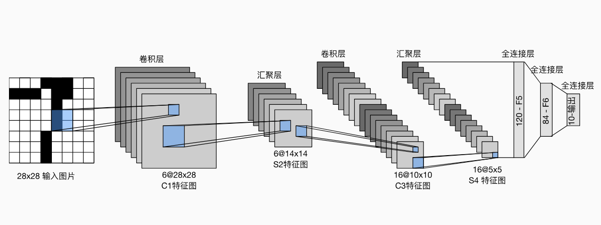
LeNet是最早发布的卷积神经网络之一,目的是识别图像中的手写数字。总体来看,LeNet(LeNet-5)由两个部分组成:
- 卷积编码器:由两个卷积层组成;
- 全连接层密集块:由三个全连接层组成。
每个卷积块中的基本单元是一个5 x 5卷积层、一个sigmoid激活函数和平均汇聚层。这些层将输入映射到多个二维特征输出,通常同时增加通道的数量。第一卷积层有6个输出通道,而第二个卷积层有16个输出通道。每个2 x 2池操作(步幅2)通过空间下采样将维数减少4倍。卷积的输出形状由批量大小(batch_size)、通道数(channel)、高度(height)、宽度(width)决定。为了将卷积块的输出传递给稠密块,我们必须在小批量中展平每个样本。换言之,我们将这个四维输入转换成全连接层所期望的二维输入。这里的二维表示的第一个维度索引小批量中的样本,第二个维度给出每个样本的平面向量表示。LeNet的稠密块有三个全连接层,分别有120、84和10个输出。因为我们在执行分类任务,所以输出层的10维对应于最后输出结果的数量。
通过下面的LeNet代码,可以看出用深度学习框架实现此类模型非常简单。我们只需要实例化一个Sequential块并将需要的层连接在一起。
import torch
from torch import nn

net = nn.Sequential(
    nn.Conv2d(1, 6, kernel_size=5, padding=2), nn.Sigmoid(),
    nn.AvgPool2d(kernel_size=2, stride=2),
    nn.Conv2d(6, 16, kernel_size=5), nn.Sigmoid(),
    nn.AvgPool2d(kernel_size=2, stride=2),
    nn.Flatten(),
    nn.Linear(16 *5 * 5, 120), nn.Sigmoid(),
    nn.Linear(120, 84), nn.Sigmoid(),
    nn.Linear(84, 10)
)
我们对原始模型做了一点小改动,去掉了最后一层的高斯激活。除此之外,这个网络与最初的LeNet-5一致。
下面,我们将一个大小为的单通道(黑白)图像通过LeNet。通过在每一层打印输出的形状,我们可以检查模型,以确保其操作与我们期望的一致。
X = torch.rand(size=(1, 1, 28, 28), dtype=torch.float32)
for layer in net:
    X = layer(X)
    print(layer.__class__.__name__,'output shape: \t',X.shape)
Conv2d output shape:         torch.Size([1, 6, 28, 28])
Sigmoid output shape:        torch.Size([1, 6, 28, 28])
AvgPool2d output shape:      torch.Size([1, 6, 14, 14])
Conv2d output shape:         torch.Size([1, 16, 10, 10])
Sigmoid output shape:        torch.Size([1, 16, 10, 10])
AvgPool2d output shape:      torch.Size([1, 16, 5, 5])
Flatten output shape:        torch.Size([1, 400])
Linear output shape:         torch.Size([1, 120])
Sigmoid output shape:        torch.Size([1, 120])
Linear output shape:         torch.Size([1, 84])
Sigmoid output shape:        torch.Size([1, 84])
Linear output shape:         torch.Size([1, 10])
请注意,在整个卷积块中,与上一层相比,每一层特征的高度和宽度都减小了。 第一个卷积层使用2个像素的填充,来补偿5x5卷积核导致的特征减少。 相反,第二个卷积层没有填充,因此高度和宽度都减少了4个像素。 随着层叠的上升,通道的数量从输入时的1个,增加到第一个卷积层之后的6个,再到第二个卷积层之后的16个。 同时,每个汇聚层的高度和宽度都减半。最后,每个全连接层减少维数,最终输出一个维数与结果分类数相匹配的输出。
模型训练
现在我们已经实现了LeNet,让我们看看LeNet在Fashion-MNIST数据集上的表现。完整代码:
import torch
from torch import nn
from torchvision import datasets, transforms
from torch.nn import functional as F
from torch.utils.data import DataLoader
import matplotlib.pyplot as plt
from matplotlib_inline import backend_inline
from IPython import display
import time

def load_data_fashion_mnist(batch_size, resize=None):
    """Download the Fashion-MNIST dataset and then load it into memory.

    Defined in :numref:`sec_utils`"""
    trans = [transforms.ToTensor()]
    if resize:
        trans.insert(0, transforms.Resize(resize))
    trans = transforms.Compose(trans)
    mnist_train = datasets.FashionMNIST(
        root="../data", train=True, transform=trans, download=True)
    mnist_test = datasets.FashionMNIST(
        root="../data", train=False, transform=trans, download=True)
    return (torch.utils.data.DataLoader(mnist_train, batch_size, shuffle=True,
                                        num_workers=4),
            torch.utils.data.DataLoader(mnist_test, batch_size, shuffle=False,
                                        num_workers=4))

class Accumulator:
    """For accumulating sums over `n` variables."""
    def __init__(self, n):
        """Defined in :numref:`sec_utils`"""
        self.data = [0.0] * n

    def add(self, *args):
        self.data = [a + float(b) for a, b in zip(self.data, args)]

    def reset(self):
        self.data = [0.0] * len(self.data)

    def __getitem__(self, idx):
        return self.data[idx]

def accuracy(y_hat, y):
    """返回预测正确的样本个数(float 类型)"""
    # 如果 y_hat 是 logits 或概率(如 [N, C]),取预测类别
    if len(y_hat.shape) > 1 and y_hat.shape[1] > 1:
        y_hat = torch.argmax(y_hat, dim=1)

    # 比较预测 vs 真实标签,并确保类型一致(避免 int64 vs int32 问题)
    cmp = (y_hat.to(y.dtype) == y)

    # 求 cmp 中 True 的个数(True=1, False=0)
    return float(cmp.sum())  # cmp.sum() 等价于 torch.sum(cmp)

def evaluate_accuracy_gpu(net, data_iter, device=None):
    if isinstance(net, nn.Module):
        net.eval()
        if not device:
            device = next(iter(net.parameters())).device
    metric = Accumulator(2)
    with torch.no_grad():
        for X, y in data_iter:
            if isinstance(X, list):
                X = [x.to(device) for x in X]
            else:
                X = X.to(device)
            y = y.to(device)
            metric.add(accuracy(net(X), y), y.numel())
    return metric[0] / metric[1]

class Animator:
    def __init__(self, xlabel = None, ylabel = None, legend = None,
                 xlim = None, ylim = None, xscale = 'linear', yscale = 'linear',
                 fmts = ('-', 'm--', 'g-.', 'r:'), nrows = 1, ncols = 1,
                 figsize = (3.5, 2.5)):
        if legend is None:
            legend = []
        backend_inline.set_matplotlib_formats('svg')
        self.fig, self.axes = plt.subplots(nrows, ncols, figsize=figsize)
        if nrows * ncols == 1:
            self.axes = [self.axes, ]
        self.config_axes = lambda: self.set_axes(self.axes[0], xlabel, ylabel, xlim, ylim, xscale, yscale, legend)
        self.X, self.Y, self.fmts = None, None, fmts
    def set_axes(self, axes, xlabel, ylabel, xlim, ylim, xscale, yscale, legend):
        axes.set_xlabel(xlabel)
        axes.set_ylabel(ylabel)
        axes.set_xlim(xlim)
        axes.set_ylim(ylim)
        axes.set_xscale(xscale)
        axes.set_yscale(yscale)
        if legend:
            axes.legend(legend)
        axes.grid()

    def add(self, x, y):
        if not hasattr(y, '__len__'):
            y = [y]
        n = len(y)
        if not hasattr(x, '__len__'):
            x = [x] * n
        if not self.X:
            self.X = [[] for _ in range(n)]
        if not self.Y:
            self.Y = [[] for _ in range(n)]
        for i, (a, b) in enumerate(zip(x, y)):
            if a is not None and b is not None:
                self.X[i].append(a)
                self.Y[i].append(b)
        self.axes[0].cla()
        for x, y, fmt in zip(self.X, self.Y, self.fmts):
            self.axes[0].plot(x, y , fmt)
        self.config_axes()
        display.display(self.fig)
        display.clear_output(wait=True)

net = nn.Sequential(
    nn.Conv2d(1, 6, kernel_size=5, padding=2), nn.Sigmoid(),
    nn.AvgPool2d(kernel_size=2, stride=2),
    nn.Conv2d(6, 16, kernel_size=5), nn.Sigmoid(),
    nn.AvgPool2d(kernel_size=2, stride=2),
    nn.Flatten(),
    nn.Linear(16 *5 * 5, 120), nn.Sigmoid(),
    nn.Linear(120, 84), nn.Sigmoid(),
    nn.Linear(84, 10)
)


def train(net, train_iter, test_iter, num_epochs, lr, device):
    def init_weights(m):
        if type(m) == nn.Linear or type(m) == nn.Conv2d:
            nn.init.xavier_uniform_(m.weight)

    net.apply(init_weights)
    print('training on', device)
    net.to(device)
    optimizer = torch.optim.SGD(net.parameters(), lr=lr)
    loss = nn.CrossEntropyLoss()
    animator = Animator(xlabel='epoch', xlim=[1, num_epochs],
                            legend=['train loss', 'train acc', 'test acc'])
    timers = []
    num_batches = len(train_iter)
    for epoch in range(num_epochs):
        metric = Accumulator(3)
        net.train()
        for i, (X, y) in enumerate(train_iter):
            timer = time.time()
            optimizer.zero_grad()
            X, y = X.to(device), y.to(device)
            y_hat = net(X)
            l = loss(y_hat, y)
            l.backward()
            optimizer.step()
            with torch.no_grad():
                metric.add(l * X.shape[0], accuracy(y_hat, y), X.shape[0])

            timers.append(time.time() - timer)
            train_l = metric[0] / metric[2]
            train_acc = metric[1] / metric[2]
            if (i + 1) % (num_batches // 5) == 0 or i == num_batches - 1:
                animator.add(epoch + (i + 1) / num_batches,
                             (train_l, train_acc, None))
        test_acc = evaluate_accuracy_gpu(net, test_iter)
        animator.add(epoch + 1, (None, None, test_acc))
        print(f'loss {train_l:.3f}, train acc {train_acc:.3f}, '
            f'test acc {test_acc:.3f}')
    print(f'{metric[2] * num_epochs / sum(timers):.1f} examples/sec '
          f'on {str(device)}')

batch_size = 256
train_iter, test_iter = load_data_fashion_mnist(batch_size=batch_size)
lr, num_epochs = 0.9, 10
train(net, train_iter, test_iter, num_epochs, lr, torch.device('cuda' if torch.cuda.is_available() else 'cpu'))
loss 0.470, train acc 0.823, test acc 0.814
141385.7 examples/sec on cuda
#